Calculate the capture zone of a well element

capzone() determines the capture zone of a well element in the flow field by performing backward particle tracking until the requested time is reached.

Usage

capzone(aem, well, time, npar = 15, dt = time/10, zstart = aem$base, ...)

Arguments

aem: aem object.
well: analytic element of class well.
time: numeric, time of the capture zone.
npar: integer, number of particles to use in the backward tracking. Defaults to 15.
dt: numeric, time step length used in the particle tracking. Defaults time / 10.
zstart: numeric value with the starting elevation of the particles. Defaults to the base of the aquifer.
...: additional arguments passed to tracelines().

Value

capzone() returns an object of class tracelines.

Details

capzone() is a thin wrapper around tracelines(). Backward particle tracking is performed using tracelines() and setting forward = FALSE. Initial particle locations are computed by equally spacing npar locations at the well radius at the zstart elevation. To obtain a sharper delineation of the capture zone envelope, try using more particles or decreasing dt.

Note that different zstart values only have an effect in models with vertical flow components.

Examples

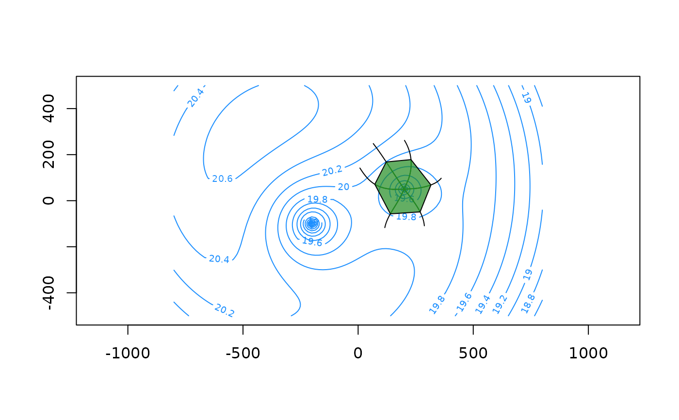
# A model with vertical flow components
k <- 10
top <- 10; base <- 0
n <- 0.3

uf <- uniformflow(TR = 100, gradient = 0.001, angle = -10)
rf <- constant(TR, xc = -1000, yc = 0, hc = 20)
w1 <- well(200, 50, Q = 250)
w2 <- well(-200, -100, Q = 450)
as <- areasink(0, 0, N = 0.001, R = 1500)

m <- aem(k, top, base, n = n, uf, rf, w1, w2, as)

# 5-year capture zone at two different starting levels
# here, the number of particles are set to small values to speed up the examples
# increase the number of particles to obtain a sharper delineation of the envelope
cp5a <- capzone(m, w1, time = 5 * 365, zstart = base, npar = 6, dt = 365 / 4)
cp5b <- capzone(m, w1, time = 5 * 365, zstart = 8, npar = 6, dt = 365 / 4)

xg <- seq(-800, 800, length = 100)
yg <- seq(-500, 500, length = 100)
contours(m, xg, yg, col = 'dodgerblue', nlevels = 20)
plot(cp5a, add = TRUE)
plot(cp5b, add = TRUE, col = 'forestgreen') # smaller zone

# plot the convex hull of the endpoints as a polygon
endp <- endpoints(cp5b)
hull <- chull(endp[, c('x', 'y')])
polygon(endp[hull, c('x', 'y')], col = adjustcolor('forestgreen', alpha.f = 0.7))